Measures of Central Tendency

Measures of Central Tendency
A frequency distribution allows us to see the overall pattern in the distribution of respondents on a variable. It is often also useful to summarize the distribution with a single number, which acts as representative. Values which locate the centre of a frequency distribution are known as measure of central tendency.
There are 3 most common measures of central tendency, the mean, the mode and the median, each appropriate for a different level of measurement.
The mean (also known as arithmetic average) is the sum of all observations divided by the number of observations. Denoted by the symbol $$\overline{x}$$ when describing a sample mean and $$\mu$$ when describing a population mean.
For the raw data, the formula for the mean is
$$\overline{x} = \frac{\sum x_i }{n}$$
If we have a frequency distribution, then the formula is
$$\overline{x} = \frac{\sum {(x_i n_i)} }{n}$$
For classified data, in calculating the mean, the above formula can be used, with x_i being the mid point of the i-th class interval and n_i being the frequency of i-th class. Also, for classified data, the following formula can be used for the mean
$$\overline{x} = x_p + \frac{h}{n} \sum_{i=1}^k {\frac{x_c-x_p}{h}n_i}$$
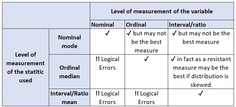
The mean is appropriate for interval/ratio level variables but not for nominal or ordinal one.
Properties of the mean:
- If the mean is subtracted from each of the measurements, the algebraic sum of these deviations is equal to zero
$$\sum_{i=1}^{n} {(x_i - \overline{x})} = 0$$
Median (may also be referred as the middle value) is the value which divides the distribution into two equal parts (the values should be ordered). Median is denoted by Me.

- If there is an odd number of observations, then the middle data point will serve as the median.
- If there are an even number of data points, the median value is assumed to be the average of the middle two values.
For classified data, the median formula is
$$Me = x_{inf} + \frac{h}{n_{Me}} (\frac{n}{2}-S_0)$$
where
x_{inf} is the lower limit of the median class;
h is the class interval of the median class;
n_{Me} is the frequency of the median class;
n is the sample/population size;
S_0 is the cumulative frequency of the class preceding the median class.
Usually, the median is more applicable when dealing with skewed data sets and/or outliers.
The median has no mathematical properties, i.e. you can not add, subtract, multiply or divide the median. It only inform us of the point in the distribution at which there are 50% of the cases above and 50% below.
Mode is the value of the observation that occurs most frequently in the distribution. Mode is denoted by Mo.
For classified data, the formula to calculate the mode is
$$Mo = x_{inf} + h \frac{n_{Mo}-n_{-1}}{2n_{Mo}-n_{-1}-n_{+1}} $$
where
x_{inf} is the lower limit of the mode class;
h is the class interval of the mode class;
n_{Mo} is the frequency of the mode class;
n_{-1} is the frequency of the class preceding the mode class;
n_{+1} is the frequency of the class succeeding the mode class.
Sometimes a distribution has more than one value with the same maximum number of observations. This is called a bimodal distribution if there are 2 modal values or multimodal if there are more modes.
The mode can be calculated for nominal, ordinal or interval-level variables, but it is the only measure of central tendency applicable to nominal variables.
Summary of measures of central tendency

There are also other central tendency measures, such as:
Midrange is the mid-point of the observations. It is calculated as the lowest observation plus the highest observation, divided in half, or
$$ Midrange = \frac{{x_{min}+x_{max}} }{2}$$
Harmonic mean is
The Geometric Mean of a sample of n positive observations is defined as the nth root of the product of the n numbers.
$$ \overline{x}_{geo} = \sqrt[n]{x_1 x_2 ... x_n} $$
Trimmed mean is a measure of central tendency calculated as the mean of the data values after "trimming" a specified percentage of the smallest and largest data values from the data set. Typically a 5% or a 10% trimmed mean is used. That way, trimmed mean is more resistant than the mean but still sensitive to specific data values.
In order to compute a 5% trimmed mean, the following steps are necessary
- Order the data from smallest to largest.
- Delete the bottom 5% and top 5% of the data. If the calculation of (0.5n) does not produce an integer, round to the nearest integer.
- Compute the mean of the remaining 90% of the data.
Observations:
- In a normal distribution, the mean, median and mode, are close to each other or equal.
- The geometric mean is used when the logarithms of the observations are distributed normally rather then the observations themselves.
- Since all values of a sample are used to calculate the mean, therefore it is the measure that is most sensitive to any change in values. Outliers can easily influence the value of the mean. This is not the case with median and mode.
- In cases with extreme values and/or skewed data, the median and the mode may be the appropriate measure of central tendency.
- Geometric mean requires positive data.
Importance of Central Tendency

